UPFINA's Mission: The pursuit of truth in finance and economics to form an unbiased view of current events in order to understand human action, its causes and effects. Read about us and our mission here.
Reading Time: 6 minutes
The central banks are about to start collectively shrinking their balance sheets. It’s the top story for the second half of 2017 and 2018 because this bull market in stocks has been pushed higher by central bank asset buying. The chart below shows how global quantitative easing pushed the market higher starting in 2009.
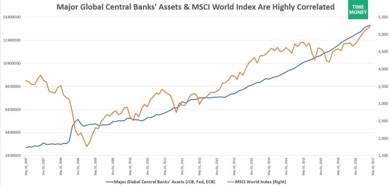
Major Global Central Banks’ Assets Versus MSCI World Index
The initial plan was to reverse panic selling, instilling confidence in the market and then to stop the asset purchases. You can think of this like a parent teaching a kid to ride a bike. The parent holds on to the seat and then releases once the kid is going fast enough. The difference in this case was the central banks didn’t let go. They’ve maintained the support for the market leading to one of the longest bull markets in history.
The problem with this policy is the wealth effect doesn’t create real growth as we have detailed previously:
The wealth effect and the whole reality of artificially creating economic demand misses one key point: If people do not have savings, and we know that asset prices cannot increase in any direction indefinitely (up or down) then what happens afterwards, when either artificially induced government demand stops, or people’s propensity to consume disappears as a function of not having savings or being maxed out on all debts?
If you’re unfamiliar, the wealth effect is when investors feel richer when their stocks go up, so they buy more goods and services. A bull market in stocks is usually a reflection of a strong economy, not something that can create a good economy. The stock market bubble in the 1990s partially made sense because of the potential of the internet. This cycle is based on the buying of central banks which is a flimsier thesis than betting on technology firms with no revenues.
The chart below shows an up to date measurement of the G-3 balance sheets which includes Japan, America, and Europe.
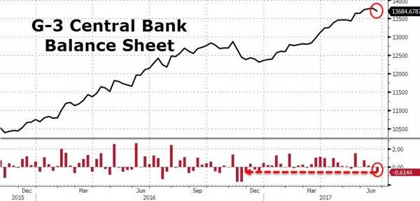
G-3 Balance Sheet Down In June
In mid-June, balance sheets shrunk the most since December. That’s only the tip of the iceberg of what’s to come. In Q3-Q4, the Fed will start to shrink the balance sheet by $10 billion per month. It will eventually raise the shrinkage to $50 billion per month. When the ECB tapers its $60 billion per month bond buying in December, the effects will really start to be felt.
The chart below shows central bank assets as a percentage of GDP, including the People’s Bank of China.
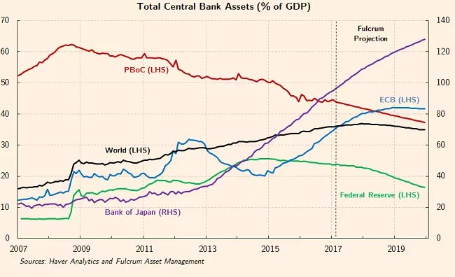
Central Bank Assets % Of GDP
The growth in the world central banks’ assets as a percentage of GDP will peak in the high 30% range and start declining in early 2018. This decline is different from previous times when there was slowing in global QE. Previous times this cycle, the rate of growth may have slowed because of a shuffling of papers between central banks of the world such as in 2010 when the PBoC shrunk its balance sheet and 2014 when the ECB shrunk its balance sheet. This time its coordinated slowing. The guidance is for shrinking which means there needs to be a real shock to the system i.e. a global recession that would reverse the current course of central bank tightening. We saw what can happen when global central banks coordinate policy in 2016 which prevented a recession in 2016.
The table below gives a summary of assumptions Fulcrum makes for the projections seen in the Total Central Banks Assets chart.
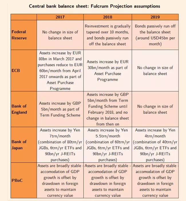
Fulcrum’s Assumptions For Global Monetary Policy
The chart above shows the Fed’s balance sheet decreasing as a percentage of GDP despite the table showing no change in the balance sheet in 2017 because the economy is growing. As was mentioned earlier, the Fed has guidance for balance sheet reductions starting in September-December 2017 which means the Fulcrum expectations are delayed more than they should be. As you can see, even the Bank of Japan, which is the most addicted to QE, is tapering its purchases in 2018 and 2019. The ECB is expected to cut its buying in half to 30 billion euros per month in 2018. The shrinkage from 80 billion per month to 60 billion per month in April 2017 was the first part of the tapering.
The interesting part comes when you try to forecast what this coordinated change in policy means for asset prices. The chart below shows what happened when the year over year growth in central bank buying stalled in 2014-2015.
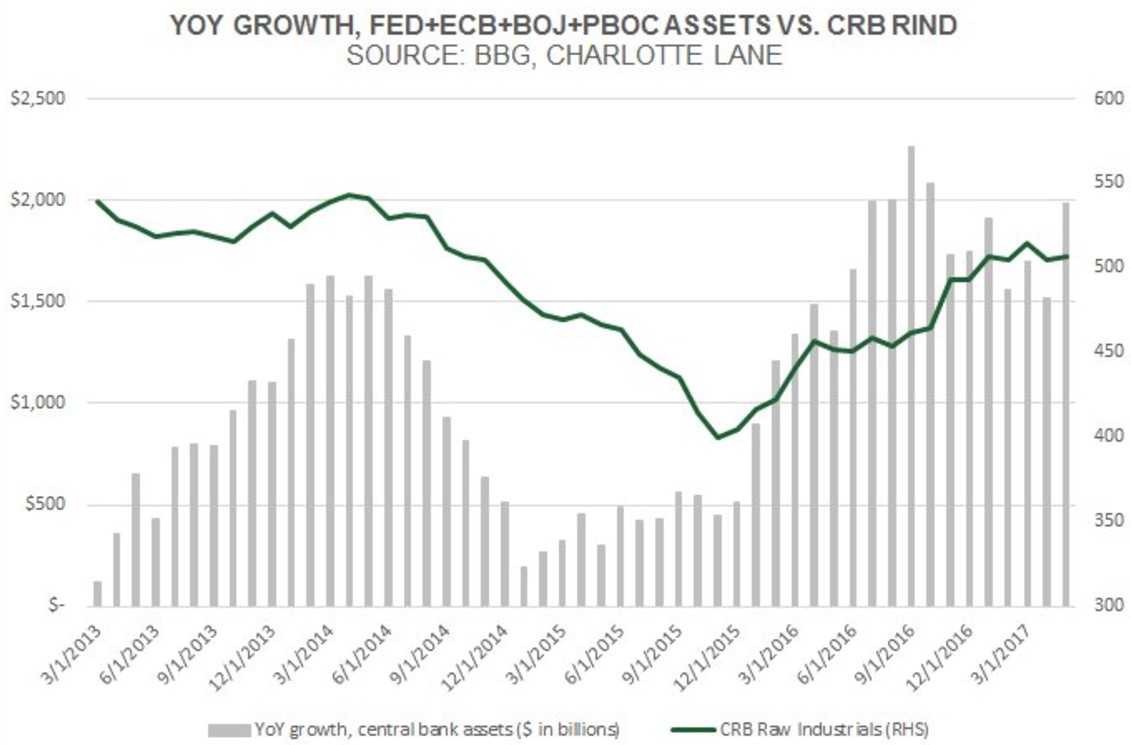
Central Bank Buying Versus CRB Industrial Commodity Index
The CRB raw industrial commodities index cratered along with decline in buying growth and then rebounded when the central banks got together to prevent a recession in early 2016. Late-2017 and 2018 will be a repeat of the decline in central banking buying, which might mean the CRB industrial commodities spot index might fall again.
If the next 18-months see commodity prices decline because of the decline in central banks’ balance sheets, it will only amplify the decline we’re already seeing in inflation. As you can see from the chart below, the May core CPI fell to 1.73% in May and core PCE fell to 1.54%.
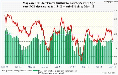
Core Inflation Already Declining
The economy is already near the inflation rate seen in 2014 before this unwind has even started which implies inflation will fall further than that. It could challenge the declines seen in the 2008 financial crisis and the environment soon afterwards.
The credit market is currently holding up well as investors continue to pile into junk bonds despite the problems in energy looking like what happened in 2014. It will be important for investors to follow the bond market for any signs of weakness caused by this global tapering. So far, the guidance for this expected tapering hasn’t caused any selling in junk bonds or stocks, but that doesn’t mean there won’t be any negative effects once it starts. The OAS seen in the chart below means options adjusted spread. It measures the difference between the risk free rate and the bond yield adjusted for an embedded option. The chart below shows how investors have fled from energy bonds, but stayed in high yield bonds which is different from 2014 when the two were highly correlated.

High Yield Versus Energy
Conclusion
Stocks have been boosted by QE since 2009. The punch bowl will be taken away in late-2017 and 2018. The last time central bank buying slowed, commodity prices crashed, pushing the entire junk bond market into a stress period. This time, instead of slowing their purchases, the central banks will shrink their balance sheets. This might have an amplified effect on commodities and risk assets. Inflation is already decreasing, so there’s no telling how low it can fall once this coordinated plan commences. The results could be continued deflation which rivals 2008. If commodity prices decline at the same rate as 2014-2015, it will start to affect the junk bond market, which would trickle into stocks, possibly spurring a selloff.
Have comments? Join the conversation on Twitter.
Disclaimer: The content on this site is for general informational and entertainment purposes only and should not be construed as financial advice. You agree that any decision you make will be based upon an independent investigation by a certified professional. Please read full disclaimer and privacy policy before reading any of our content.